$$ \definecolor{myBlue}{RGB}{255, 196, 87} \newcommand{\info}[1]{{\color{myBlue} #1}} \newcommand{\svec}{\boldsymbol} \newcommand{\bu}{\svec{u}} \newcommand{\bJ}{\svec{J}} \newcommand{\R}{\mathbb{R}} \newcommand{\Rtwo}{{\R^2}} \newcommand{\Rthree}{{\R^3}} \newcommand{\H}{\mathcal{H}} \newcommand{\M}{\mathcal{M}} \newcommand{\U}{\mathcal{U}} \newcommand{\prt}[1]{\left(#1\right)} \newcommand{\brk}[1]{\left[#1\right]} \newcommand{\abs}[1]{\left|#1\right|} \newcommand{\norm}[1]{\left\|#1\right\|} \newcommand{\inner}[1]{\left\langle#1\right\rangle} \newcommand{\grad}{\nabla} \newcommand{\gradx}{\grad_x} \newcommand{\gradv}{\grad_v} \newcommand{\vs}{v_*} \newcommand{\xs}{x_*} \newcommand{\gradvs}{\grad_{\vs}} \newcommand{\div}{\grad\cdot} \newcommand{\divx}{\gradx\cdot} \newcommand{\divv}{\gradv\cdot} \newcommand{\divvs}{\gradvs\cdot} \newcommand{\curl}{\grad\times} \newcommand{\curlx}{\gradx\times} \newcommand{\curlv}{\gradv\times} \newcommand{\laplacian}{\Delta} \newcommand{\laplace}{\laplacian} \newcommand{\laplacex}{\laplacian_x} \newcommand{\laplacev}{\laplacian_v} \newcommand{\conv}{\ast} \renewcommand{\star}{\conv} \newcommand{\convx}{\conv_{x}} \newcommand{\convv}{\conv_{v}} \newcommand{\convxv}{\conv_{x,v}} \renewcommand{\d}{\mathrm{d}} \newcommand{\dd}{\mathop{}\!\d} \newcommand{\dt}{\dd t} \newcommand{\dx}{\dd x} \newcommand{\dy}{\dd y} \newcommand{\dv}{\dd v} \newcommand{\dw}{\dd w} \newcommand{\dvs}{\dd \vs} \newcommand{\dxs}{\dd \xs} \newcommand{\Dt}{\Delta t} \newcommand{\Dx}{\Delta x} \newcommand{\Dy}{\Delta y} \newcommand{\der}[2]{\frac{\d #1}{\d #2}} \newcommand{\pder}[2]{\frac{\partial #1}{\partial #2}} \newcommand{\secondpder}[2]{\frac{\partial^2 #1}{\partial #2^2}} \newcommand{\doublepder}[3]{\frac{\partial^2 #1}{\partial #2 \partial #3}} \newcommand{\vder}[2]{\frac{\delta #1}{\delta #2}} \newcommand{\pt}{\partial_t} \newcommand{\px}{\partial_x} \newcommand{\pxx}{\partial_{xx}} \newcommand{\p}{_{p}} \newcommand{\q}{_{q}} \newcommand{\pq}{_{p,\,q}} \newcommand{\Np}{N} \newcommand{\Nc}{N_c} \newcommand{\Nx}{N_{x}} \newcommand{\Ny}{N_{y}} \newcommand{\Nz}{N_{z}} \newcommand{\Nv}{N_{v}} \newcommand{\Nvx}{N_{v_x}} \newcommand{\Nvy}{N_{v_y}} \newcommand{\Nvz}{N_{v_z}} \newcommand{\Nb}{N_b} \newcommand{\fN}{f^\Np} \newcommand{\ftN}{\tilde{f}^\Np} \newcommand{\tH}{\tilde{\H}} \newcommand{\U}{\mathcal{U}} \newcommand{\ex}{\eta} \newcommand{\ev}{\varepsilon} \newcommand{\Sx}{\psi_\ex} \newcommand{\Sv}{\varphi_\ev} \newcommand{\convx}{\conv_{x}} \newcommand{\convv}{\conv_{v}} \newcommand{\convxv}{\conv_{x,v}} \newcommand{\rhomax}{\rho_{\text{max}}} \newcommand{\eps}{\varepsilon} \newcommand{\n}{^{n}} \newcommand{\np}{^{n+1}} \newcommand{\i}{_{i}} \newcommand{\ip}{_{i+1}} \newcommand{\ih}{_{i+1/2}} \newcommand{\imh}{_{i-1/2}} \newcommand{\pos}[1]{\prt{#1}^+} \newcommand{\neg}[1]{\prt{#1}^-} \newcommand{\bE}{\mathbb{E}} \newcommand{\bR}{\mathbb{R}} \newcommand{\bW}{\mathbb{W}} \newcommand{\cE}{\mathcal{E}} \newcommand{\cP}{\mathcal{P}} \newcommand{\cW}{\mathcal{W}} $$

Data-Driven Computational Science


Centre for Analysis,
Scientific Computing,
and Applications

Rafael Bailo
Olga Mula

Benjamin
Caris

Daan
Bon
Federico
Vismara
Pratik
Rai

How do we think about these problems?

1: The Forward Problem

We make a mathematical model: We write down differential equations (ODEs, PDEs) that approximately describe the system we want to study.

These equations usually depend on parameters which control the overall behaviour of the system.

For example, a simple model for pedestrians is$$ \dot{x}_i = v_i + c \sum_{j\neq i} F(x_i,x_j). $$

  • $x_i$ is the position of the ith pedestrian.
  • $v_i$ is the desired velocity of the ith pedestrian.
  • $F$ is some repulsive force .
  • $c$ is a parameter that controls the strenght of repulsion.

Simulation

2: The Inverse Problem

We now calibrate the model to match the real world. We try to find the best parameters.

We do this automatically by solving an optimisation problem. Usually, we are comparing the model with real-world data.

3: Model Discovery

Even after calibration, is our model the right model?

Can we discover a mathematical model automatically, directly from data?

In the pedestrian model, could we replace the force by a neural network?$$ \dot{x}_i = v_i + \sum_{j\neq i} NN(x_i,x_j). $$

Could we replace the whole model by a neural differential equation?$$ \dot{x}_i = NN(x_i; x_1,x_2,\cdots). $$

What tools do we use?

PDEs + Data

  • (Partial) differential equations
  • Machine learning
  • Optimisation
  • Numerical analysis
  • Reduced order models
  • Optimal transport
  • Inverse problems
  • High-performance computing

Relevant Courses

  • Q1: 2MMD10
    Optimisation
  • Q1: 2MMN10
    Scientific computing
  • Q2: 2MMA10
    Applied functional analysis
  • Q2: 2MMA80
    Mathematics of neural networks
  • Q3: 2MMA20
    Partial differential equations
  • Q4: 2MMN30
    Scientific computing in PDEs

Examples of dissertation projects we offer

Rafael's past project:

Hydrodynamic Modelling of Pedestrian Flow in a Corridor

Rafael's upcoming project:

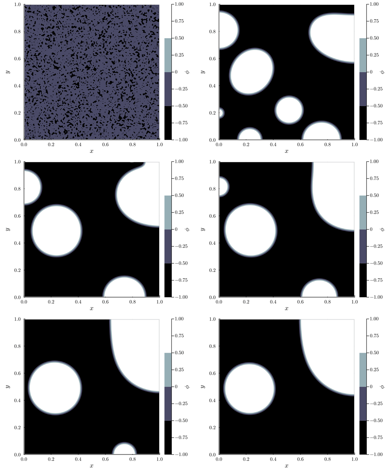
Structure Preserving Simulation of Crystal Growth
Rafael's upcoming project:

Neural Networks for Pedestrian Dynamics

Olga's past project:

Estimation of Blood Flow in the Carotid Artery

Olgas's upcoming project:

PINNs for the Radiative Transfer Equation

Olgas's upcoming project:

Inverse Problems for Wasserstein Gradient Flows

Questions? Get in touch!

Rafael Bailo rafaelbailo.com r.bailo@tue.nl
Olga Mula omula.gitlab.io o.mula@tue.nl